Python Data Analysis on Japanese Adult Video (JAV) dataset

I have been working with Python for sometimes. Most of the time I build the machine learning API and spend times playing with algorithms, I haven’t seriously taking the Analysis part. I taught myself for data analysis through courses, video,..etc.. and it comes a time I think that I have to do something. Well, practising always better than studying.

I have been searching the dataset for a while, a dataset which is not so simple, not so complicated and fun to play around. Then one of my friend, he suggests me the JAV idols dataset which he scraping from DMM website (thanks Harry Pham).

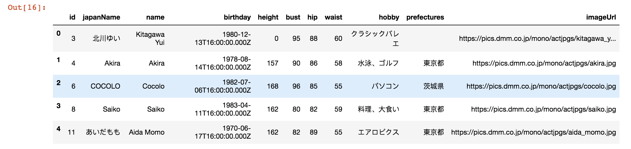
The first dataset is the list of actresses. Which has the features: id , japanName , name , birthday , height , bust , hip , waist , prefectures and imageUrl.

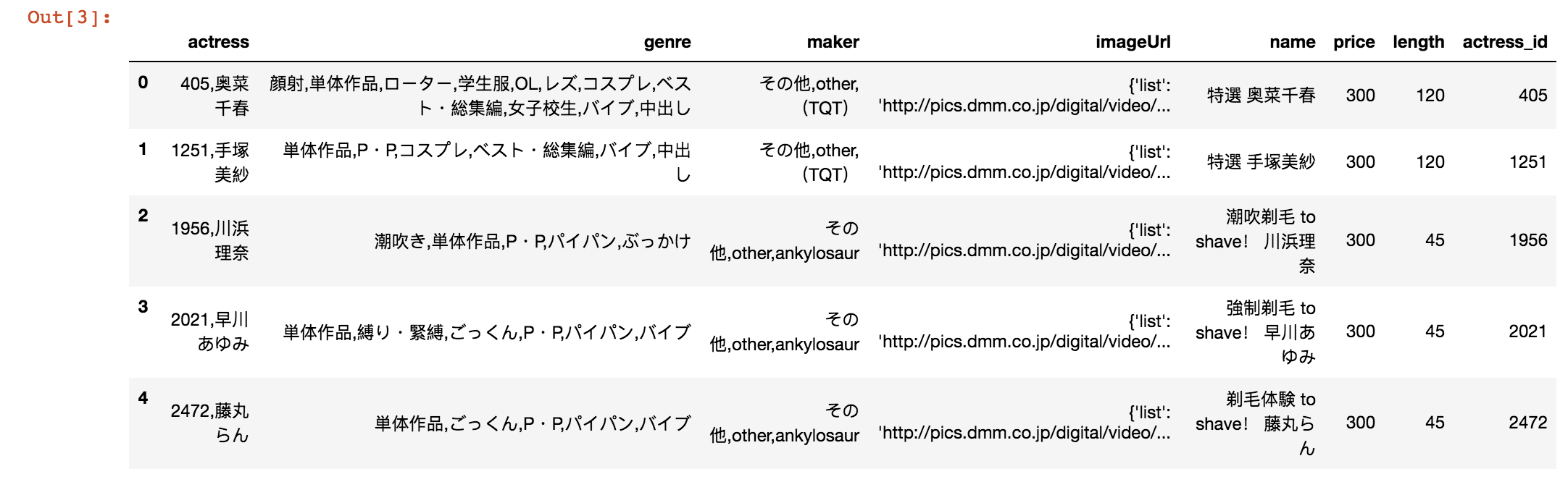
The second dataset is a list of movies with actress , genre , maker , ImageUrl , name , price , length , actress_id

Well, to be honest, it took me quite time to decide what can I do with these two datasets. Then I came up with the idea combine both two together. And mostly focus on the the actresses data.

Here is what I’ve done

From the movies dataset, I’m counting the number of movies and number of genres for single particular actress.

Counting number of movies:

def _counting_movies(actress_id):
    return len(train_movie[train_movie.actress_id == actress_id])
train_actress['no_movies'] = train_actress['id'].apply(lambda x: _counting_movies(x))

_Counting number of genres:

def _counting_genre(actress_id):
    actress_info = train_movie[train_movie.actress_id == actress_id]
    return len(list(set(','.join(actress_info['genre']).split(','))))
train_actress['no_genres'] = train_actress['id'].apply(lambda x: _counting_genre(x))

With the actress dataset, I write a small codes to get the age of each actress

train_actress['birthday'] = pd.to_datetime(train_actress['birthday'])
train_actress['age'] = train_actress['birthday'].apply(lambda x: pd.to_datetime('today').year - x.year)

The final dataset will look like

<class 'pandas.core.frame.DataFrame'>
Int64Index: 3664 entries, 0 to 10156
Data columns (total 12 columns):
id             3664 non-null int64
name           3664 non-null object
bust           3664 non-null int64
waist          3664 non-null int64
hip            3664 non-null int64
birthday       3664 non-null datetime64[ns]
age            3664 non-null int64
hobby          2856 non-null object
prefectures    2712 non-null object
no_movies      3664 non-null int64
no_genres      3664 non-null int64
imageUrl       3664 non-null object
dtypes: datetime64[ns](1), int64(7), object(4)
memory usage: 372.1+ KB

I can see there are 3664 entries, and the values of columns are int64, object or datetime64 mean string, integer and datetime. For prefectures variable, there are only 2712 non-null entries, which means there are 952 missing values. Missing values needs to be handled cautiously. There might be a reason why they are missing, and you might find some useful insight by figuring out the reason. Sometimes missing part might even distort the whole data. But for this case, prefectures is not an significant variable so I will leave it.

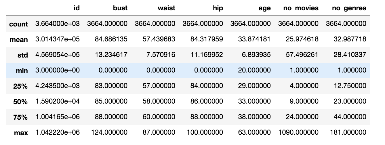
Now it’s time for some small EDA (Explanation Data Analysis). I will do with a small statistic with numerical variables first

Let’s move on with some useful inside about BUST.

I do a quick sort by using .sort_value() function and tackle it with df.head() function to get the first 5 records.

df = df.sort_values(by="bust", ascending=False)
df.head()

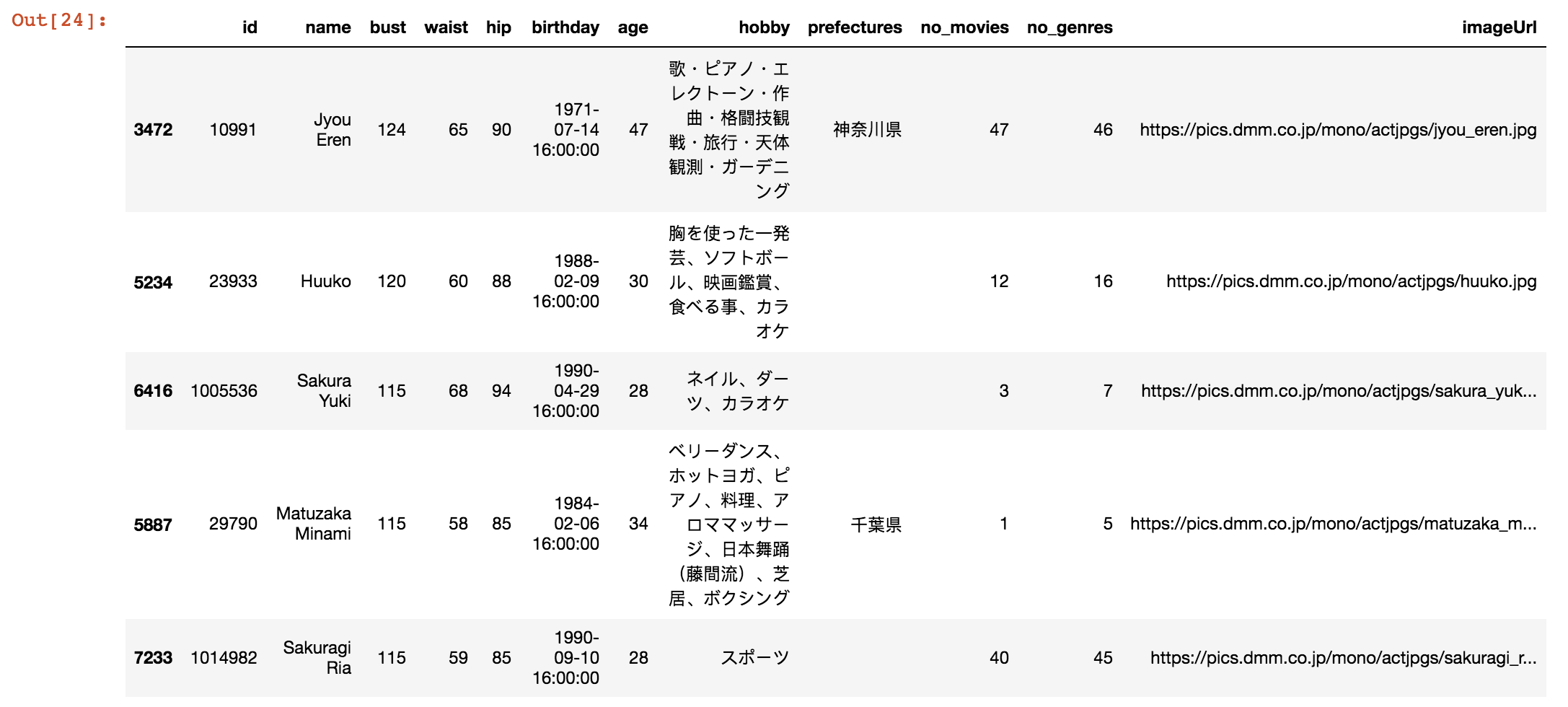
The actress has the biggest bust size (124) is Jyou Eren. For your information, here is the picture of her.

Well she’s 47 years old now and she already retired, so we cannot expect much right. You guy also can check the actress with the smallest bust size by using the df.tail() . Hint the smallest size in this dataset is 65 (you can check it on my notebook link below the article)

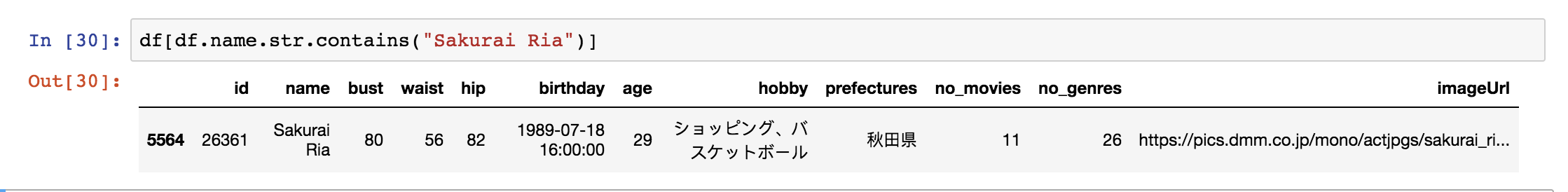
Finally, to verify the dataset, I check one of the famous actress whom I know. Her name is Ria Sakurai.

Coming up, I think I will do something different, more complex but still related to the bust. Let’s see how bust size differ from age to age, it is a good ideal to group age into category . By using the seaborn I can visualize the age distribution

sns.set(color_codes=True)
sns.distplot(df['age']);

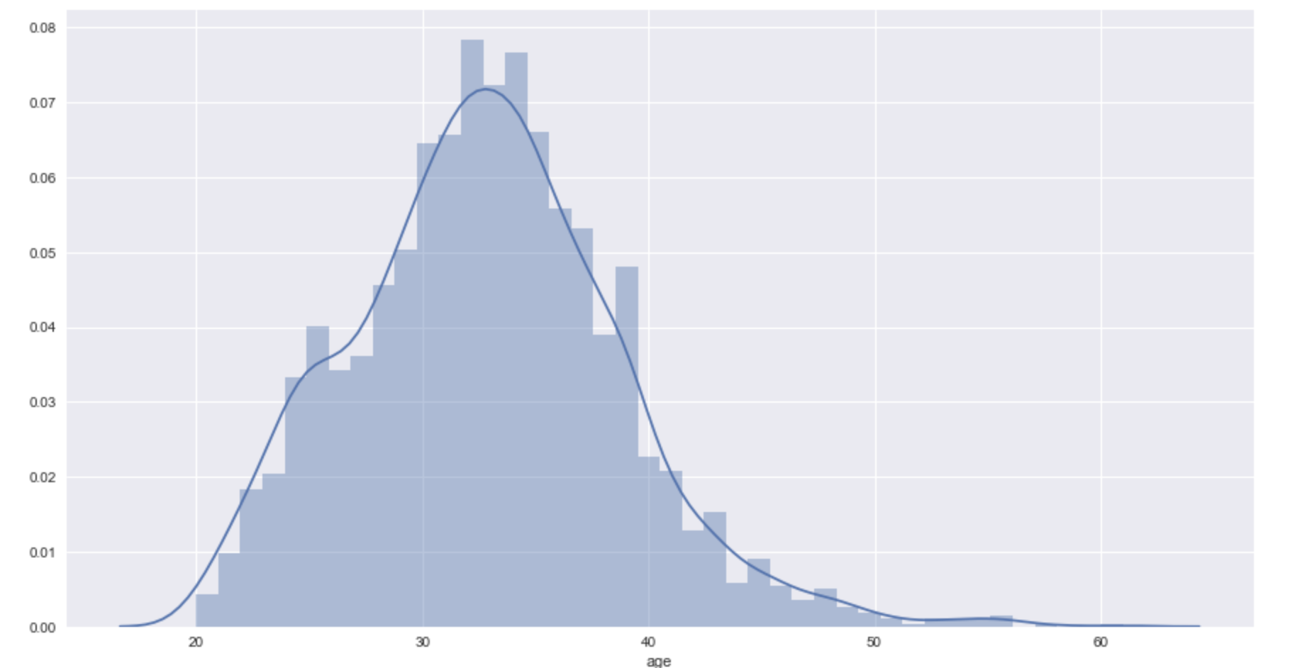
Most of actresses in the dataset is between 30 and 40 years old. So I make a new column call age_cat for categorise the age.

df['age_cat'] = pd.cut(df['age'], bins=[20, 30, 40, float('Inf')], labels=['A', 'B', 'C'])
# A will be between 20 years old
# B will be between 30 and 40 year old
# C will be 40 and above

I use violin plot to see the “bust size” distributed across the ages

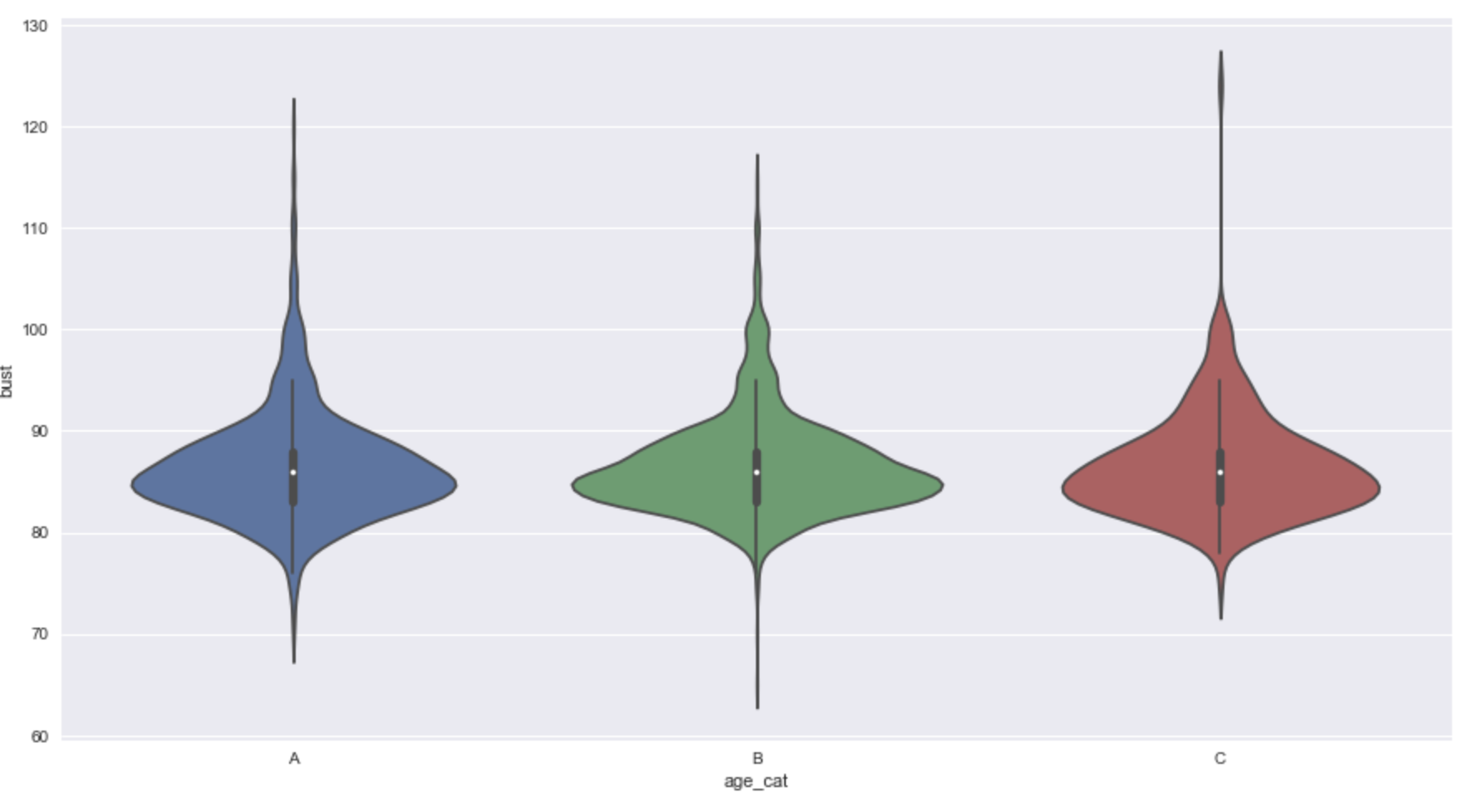
It looks like cat A (from 20 to 30) is more dispersed than others, while cat B (from 30 to 40) looks the shortest with two distinctive peaks. At least, from the plot, it looks like there not much significant difference between ages, but too early to tell.

My extra work, I find more information beside bust from the dataset.

With the hobby, I will use wordcloud library to visualise the top activities that actresses usually do in their leisure

wordcloud = WordCloud(
        max_words=200,
        max_font_size=40, 
        scale=3,
        random_state=1 
    ).generate(hobby)

My Japanese are not good, but enough to tell some in here. Most of the leisure activities are Karaoke (カラオケ), Shopping (ショッピング), cooking (料理), swimming (水泳) and piano (ピアノ).

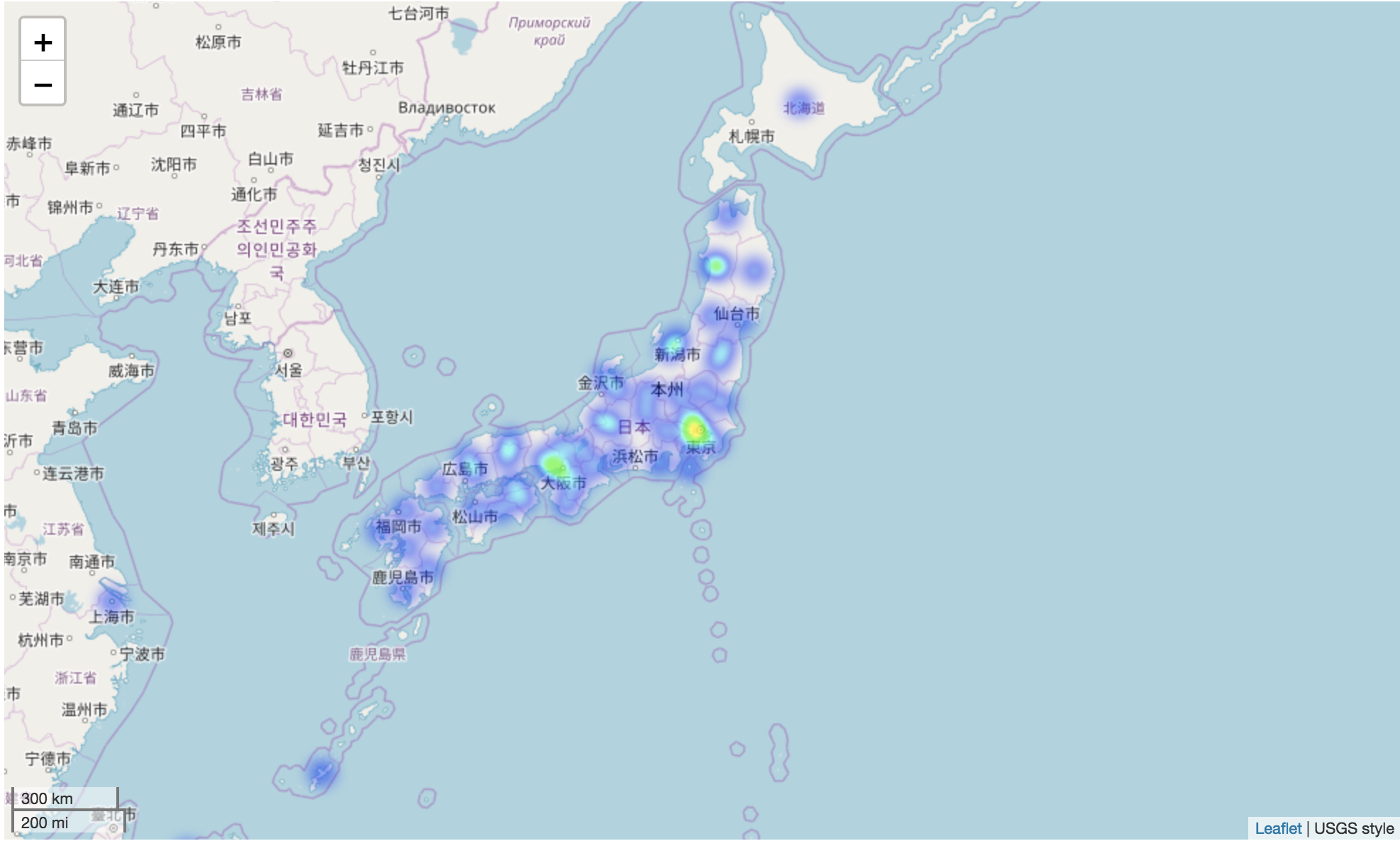
There still one more interesting column in the dataset prefectures . I want to see which areas of Japan has the most actresses was born.

To visualise the location on the map, I have to convert the location name to longitude and latitude. geopy library is good enough for me instead of google map api.

from geopy.geocoders import Nominatim
import time
geolocator = Nominatim()

# Get latitude and longitude by using city name
def get_location(adress):
    location = geolocator.geocode(adress)
    return location.latitude, location.longitude

# Get lat and lng
prefecture_df['location'] = 1
for index, row in prefecture_df.iterrows():
    count = 0
    while count < 5:
        try:
            prefecture_df.loc[index,'location'] = str(get_location(row['prefectures']))
            count = 6
        except:
            count += 1
    time.sleep(5)

After filter the prefecture to a new dataset with latitude and longitude. I use the folium library to show it on the map.

I think that all for this post. If you want to get more details, please find the code in my Github (https://github.com/canhtran/jav_idol_analysis).